Fast markets need fast indicators. One of these indicators is the Double Exponential Moving Average (DEMA), made to meet this need. It reduces lag, allowing quicker reaction to price movements. By smoothing out the price data while staying responsive to changes, it helps in revealing the trend direction and identifying entry and exit points. In this guide, we’ll explore how the DEMA works and understand its application in trading.
What is the Double Exponential Moving Average (DEMA)?
In technical analysis, the Double Exponential Moving Average (DEMA) was created to reduce signal lag. Patrick Mulloy developed it in 1994 with the purpose to react more quickly to the price movement.
Moving averages smooth out the price data to reveal the trend. But the drawback of many moving averages is that they respond slowly to sudden price changes. The DEMA addresses this problem. It responds quickly to price change but still maintains smoothness.
Because it reacts faster, it may help in early identification of trend reversals or breakout opportunities.
How the Double Exponential Moving Average Works
The DEMA works by combining two Exponential Moving Averages (EMAs) in a way that removes much of the lag seen in standard averages.
Firstly, an EMA for the specified time period is calculated. Then this value is used to calculate the second EMA. The DEMA formula uses both values to produce a smoother and faster line that closely follows the price action.
The DEMA is plotted on the chart to identify the trend. If the price stays above the DEMA, it reflects bullish momentum. If the price drops below, it signals growing bearish sentiment.
However, like all indicators, the DEMA works best when used alongside other tools such as volume analysis, momentum indicators, or support and resistance levels.
Examples of DEMA
The Double Exponential Moving Average can be applied in real trading scenarios to observe how the price interacts with the indicator. The following Nifty 50 chart for January 2026 to February 2026 shows how the DEMA works:
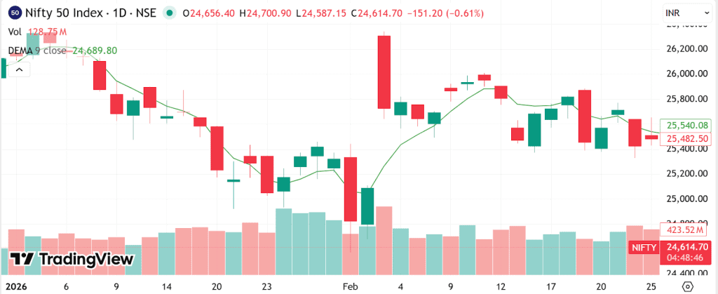
- In early January 2026, the Nifty 50 was moving around 26,000, and DEMA was closely following it at the same levels.
- On January 21, 2026, the Nifty dropped close to 25,100 below the DEMA line, which was at 25, 300.
- By the end of January, buyers started to step in. The price started moving back toward the DEMA line, suggesting a possible short-term stabilisation.
- In February, the Nifty had a strong rally and touched 26,300 on February 3, 2026, significantly above the DEMA at 25,267. This confirmed the bullish momentum.
- In the next sessions, the Nifty 50 fluctuated around the 25,500 mark. The DEMA line also stayed more or less aligned with the momentum.
- The Nifty 50 finally dropped to 25,482, below the DEMA at 25,540 on February 25, suggesting growing bearish pressure.
Calculating the Double Exponential Moving Average (DEMA)
The formula for calculating the DEMA is calculated is as following:
DEMA(n)=2×EMA(n)−EMA(EMA(n))
Where n is the number of periods used
DEMA(n) – Double Exponential Moving Average for period n
EMA(n) – Exponential Moving Average calculated over n periods
This formula may look complex at first, but it simply adjusts a regular exponential moving average so that it reacts faster to price changes.
Let’s understand the calculation with a hypothetical example:
Assume a trader is using a 5-period DEMA, and we already calculated the EMA values.
Step 1: Calculate the first EMA
Suppose the 5-period EMA of a stock price is:
EMA(n) = 50
Step 2: Apply the EMA calculation again
Next, we calculate another EMA using the first EMA values.
EMA(EMA(n)) = 48
Step 3: Substitute values in the DEMA formula
DEMA = 2 × EMA(n) − EMA(EMA(n))
DEMA = 2 × 50 − 48
DEMA = 100 − 48 = 52
In this example, the EMA value was 50, but the DEMA became 52, reflecting its faster response to price changes.
Applications of the Double Exponential Moving Average
The DEMA is mainly used to understand market direction and price behaviour. Traders use it to analyse trends and identify potential trading zones.
Trend Analysis
The most common use of the DEMA is to confirm whether a market is trending upward or downward.
- When the price consistently stays above the DEMA line, it indicates that the momentum is upward and buying pressure is increasing.
- On the other hand, the prices staying below the DEMA suggest sellers taking control and point to a downward trend.
You can use this to align your positions with the broader trend and avoid trading against the market direction.
Support and Resistance
The indicator may also function as a dynamic support or resistance zone.
- In an uptrend, the prices sometimes pull back toward the DEMA line before moving higher. The DEMA can act like a support area.
- During a downtrend, the DEMA becomes the resistance level where the price struggles to move beyond it.
These levels help in determining potential entry and exit points.
Difference Between EMA and DEMA
The given table compares the difference between the DEMA and the Exponential Moving Average (EMA):
| Feature | EMA | DEMA |
| Indicator Type | Single exponential moving average indicator | Double smoothed exponential average indicator |
| Lag | Moderate lag during strong trends | Reduced lag for quicker signals |
| Reaction Speed | Responds moderately to recent prices | Responds faster to price movement |
| Calculation | Single smoothing exponential formula | Combines two exponential averages |
| Common Use | Basic trend following strategies | Faster momentum trend strategies |
Advantages of Using DEMA
There are several benefits that make the DEMA appealing to traders.
- Faster Signals: As the DEMA reduces lag, it can generate signals faster than other moving averages.
- Better Trend Clarity: It closely tracks and responds to price movements, which makes identifying the trend direction easier.
- Flexible Use: DEMA can be used in various strategies, including trend-following, crossover systems, and momentum analysis.
- Improved Noise Filtering: Although being fast, the DEMA still smooths out the price fluctuations, which filters the noise and results in fewer false signals.
- Compatibility: Using other tools like MACD, volume or RSI, MACD, strengthen the signals produced by the DEMA.
Disadvantages of Using DEMA
Despite its advantages, the DEMA also has limitations that should be considered.
- Unsuitability for Ranging Markets: In sideways markets, the indicator crosses the price frequently, which does not lead to any meaningful trends.
- High Sensitivity: As the DEMA reacts quickly to the price changes, it can create false signals in choppy markets, trapping the traders.
- Requires Confirmation: The indicator is dependent on other confirmation tools and should not be used in isolation.
- Learning Curve: The DEMA is complex in nature as compared to other moving averages. Beginners may find it hard to apply and interpret this indicator.
- Overtrading: Due to its quick nature, traders might receive too many signals, leading to many unfavourable trades and higher transaction costs.
Conclusion
By combining two EMAs, the DEMA provides a smoother yet faster response to the price momentum. The DEMA helps in identifying the trend and planning trade positions. Like any other technical indicator, it should not be used as a standalone. Combining it with volume, RSI, MACD, or other tools improves its accuracy and results in better trading results.
Understanding how and when to use the DEMA improves analysis and allows easy navigation of the market trends.
FAQs
The EMA uses a single exponential smoothing calculation that gives more weight to recent prices. The double EMA applies the exponential smoothing process twice to reduce lag and produce faster trend signals.
A common strategy is to use two DEMA lines with different time periods. Traders often look for crossovers between the short-term and long-term DEMA to identify potential buying or selling opportunities.
Double exponential smoothing is useful when traders want faster signals and reduced lag compared to traditional moving averages. It is often used in trending markets where quick responses to price changes are important.
Double exponential smoothing is also known as Holt’s linear trend model or Holt’s method. It was developed by Charles Holt to extend simple exponential smoothing to support data with linear trends.